1. Physical system

A random spectrometer as shown in Fig. 1 is made of random air holes on top of a silicon substrate. Since the position of airholes are random, the details of individual modes and their frequencies are not important, therefore, we can focus on the statistical properties of the system given the number of modes and a coupling matrix.

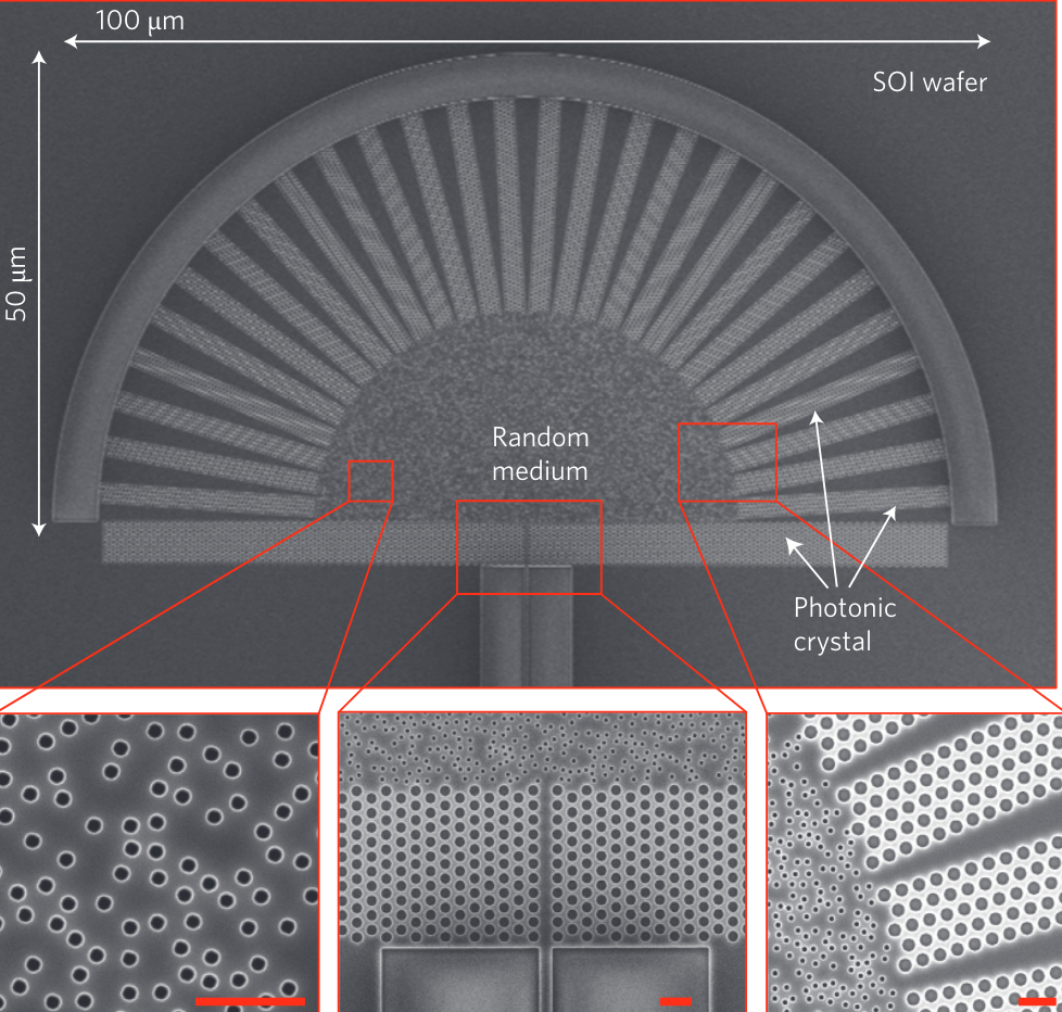SEM image of random spectrometers Figure 1: SEM image of frabricated random spectrometers. Figure adapted from Ref. [1].

Luckily, in mathematics we have Random matrix theory (RMT) which are used to desribe statistics of eigenfrequencies and associated eigenfunctions. Since in spectrometers the most important properties we care about is the resolution which basically can be represented as the correlation function.

1.1 General description

Assuming that exactly $M$ channels at given energy $E$ are “open” (Allow for an unbounded motion of the particles), we associate with the channel region a continuous set of functions $|a,E \rangle, a = 1,…,M$ normalized as $\langle a, E_1|b, E_2 \rangle = \delta_{ab} \delta(E_1-E_2)$. An analogous, but discrete set of orthogonal states $|n\rangle, n = 1,2,…,N$ is associated with the compact interaction region.

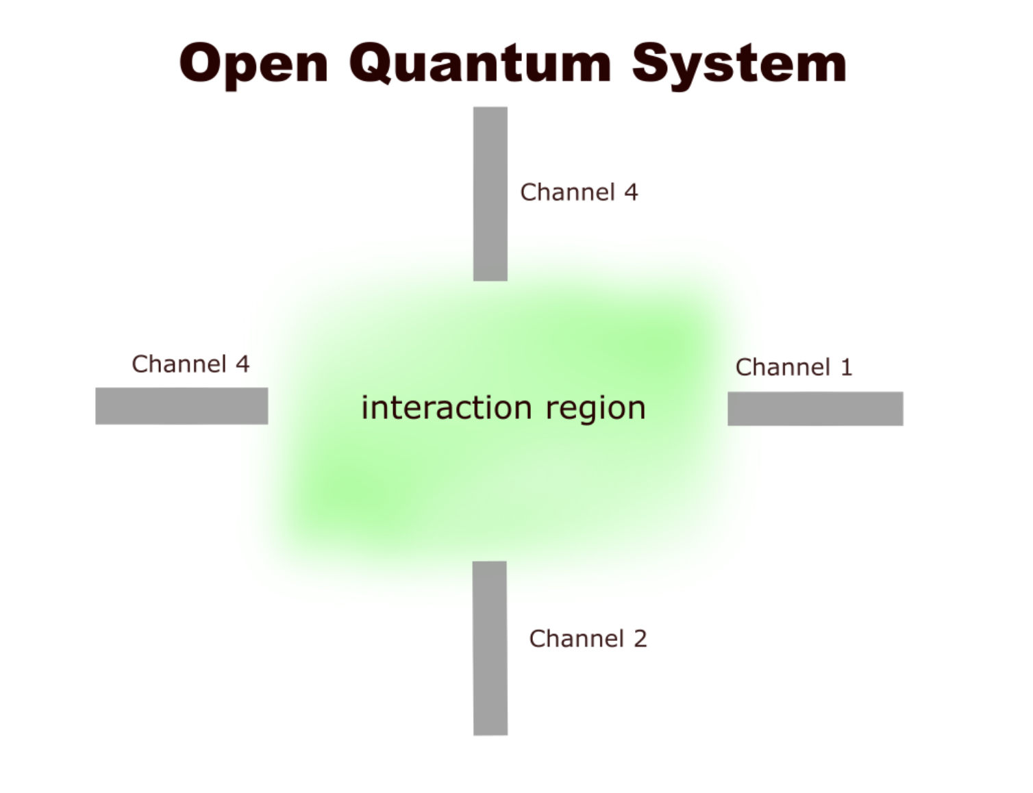Open quantum system Figure 2: Interaction region (channels of reaction)

Without any interaction, the Hamiltonian of the system is: $$H_0 = \sum_{l,m} |l \rangle (H_{in})_{l,m} \langle m| + \sum_a \int dE |a,E\rangle E \langle a,E|$$

where the integration goes over the energy region where the give channel $a$ is open.

Now we simulate $H_{in}$ as a Gaussian random $N\times N$ matrix and $N \gg 1$.

而interaction term可以表述为：

$$V = \sum_{l,a} (|l\rangle \int dE W_{la}\langle a,E| + h.c.)$$

这里要保证total Hamiltonian $H = H_0 + V$为self-adjoint （对于bound states就是Hermitian了）

写到这一步就可以进入Scattering theory的标准程序了。也就是写下Lipmann-Schwinger equation然后计算scattering matrix。

Incoming wave amplitudes $A = (A_1, …, A_M)^T$, outgoing wave amplitudes $B = (B_1, …, B_M)^T$ $$B = \hat S A$$ $S$ is unitary to make sure the conservation of the probability flux. $SS^\dag = I$ S的共轭转置代表输入和输出互换。所以unitary的意思就是 $S^\dag B = S^\dag SA = A$, 整个过程中没有额外的能量损耗。

1.2 Weak coupling regime

When W -> 0, the anti-Hermitian part $-iWW^+$ can be treated as a perturbation of the Hermitian part. The resonance of $H_{eff}$ is the close to hermitian $H$ which is real energy $E$. In this regime one expects the resonances to be largely non-overlapping.

The mean space between neighbouring real eigenvalues $\Delta$ is known to obey the Porter-Thomas distribution. 这种能隙距离的分布不就恰好能够说明correlation length的变化吗？也就是说当平均能隙距离$\Delta$变小的时候，系统就具备更小的resonance间距。

The relation between resonance and correlation length

（mean density of resonances) The number of resonances is equal to N. While the overlapping between resonances will definitely affect the correlation length.

“Lifetime statistics of quantum chaos studied by a multiscale analysis” This paper seems to be quite useful for understanding resonances in spectrometer.

2. RMT parameters

The $M\times M$ scattering matrix $S(E)$ for a random media with $M$ open channels can be represented by:

$$S(E) = I - iW^{\dag}\frac{1}{E-H_{eff}}W, \quad H_{eff} = H - \frac{i}{2}WW^{\dag}$$

Where $H$ is a $N \times N$ Gaussian unitary ensemble, The effective non-Hermitian hamiltonian $H_{eff} = H - i/2 T, T = WW^\dag$ has N complex eigenvalues $z_n = E_n - iT_n/2$, which provide poles of the scattering matrix in the complex energy plane, commonly refer to as the resonance.

$W = t_{coupling} * W_0$ is a $N\times M$ matrix represents coupling amplitudes to M open scattering channel.

The columns of $N\times M$ matrix W of coupling amplitudes to M open scattering channels can be taken either as fixed orthogonal vectors satisfying $∑^N_{i=1} W_{ai}W_{bi} = γ_aδ_{ab}, γ_a > 0 ∀a = 1, . . . , M$ or alternatively the entries are chosen to be independent random Gaussian: $i, j = 1, . . . , N$, with angular brackets standing for the ensemble averaging. Origin source: Random Matrix Theory of Resonances: an Overview

Finally, we have the transmission matrix: $$T(E) = abs(S(E)[1:M, 0])$$

Therefore, we have several parameters here: $t_{coupling}$: the coeffeicient for W $N$: number of modes, the size of H $NFC$: number of frequency channels, the number of E samples.

Next, we derive from scattering matrix to transmission matrix

The transmission matrix is defined by the relation between input signal intensity $x$ and output detector intensity $y$: $$y = T\cdot x$$

While the input signal amplitude $A_x$ and output detector amplitude $A_y$ is connected by the scattering matrix:

$$A_y = \Sigma_E S(E) A_x$$

($T(E) = abs(S(E)[1:M, 0])$ is not correct. How to derive the correct form?)

E[1:M,0] can be rewrite as a product of projector vector $P_M$ and S(E):

$$T(E) = P_M (S^*(E)S(E))^{1/2}$$

$S^*(E)$ is the complex conjugate form of $S(E)$.

$P_M$ basically means the projection of S(E) to the 1:M column of S(E).

3. Python implementation

Next, we are going to implement the simulated spectrometer in python and generate the transmission matrix for machine learning training.

The first step is to generate model Hamiltonian $H$. $H$ is a $N \times N$ Gaussian unitary ensemble (GUE), representing model spectral properties of the Hamiltonian of the spectrometer.

$$H = \frac{1}{2}(A + A^\dag)$$

def GUE(N):
    A = np.random.normal(0,1,(N,N)) + 1j*np.random.normal(0,1,(N,N))
    H = 0.5*(A + A.conj().T)
    return H

Next we construct the S-matrix according to the formula below:

$$S(E) = I - iW^{\dag}\frac{1}{E-H_{eff}}W, \quad H_{eff} = H - \frac{i}{2}WW^{\dag}$$

####  Construct a S-matrix
def S_matrix(params, E0 = 0.0):
    
    H = GUE(N)    
    W = t_coupling*np.random.normal(0, 1, (N, M))
    
    I = np.identity(M)
    E = E0*np.identity(N)
    T = W@W.T
    H_eff = H - 1j*T
    SE = I- 2*1j*W.T@inv(E-H_eff)@W
    
    return np.abs(SE)
    # return SE

I think the way we generate the W matrix is not correct. I used a gaussian distribution for this. I should double check it. W matrix 应该是一个加起来等于多少的矩阵，而不是直接用一个gaussian来代替？

In principle, S-matrix should be a complex non-Hermitian matrix dependent of energy E. But here I take the absolute value for S(E) because I think for the detector we only care about the intensity.

How do we take. the value for E0 by the way, is it correct?

Then the generation of Transmission matrix:

def generate_transmission_matrix(params, NFC, energy_span, trans_matrix_location):

    trans = []
    
    M = params['M']
    
    for E0 in energy_span:
        SE = S_matrix1(params, E0 = E0)
        trans.append(SE[0,1:M])
    
    trans = np.array(trans)

    with open(trans_matrix_location, 'wb') as f:
        pickle.dump(trans, f)
            
    return trans.T

4. Differentiate Transmission matrix

End-to-end optimization对于RMT 来说好像也可以公式化地推导出来，对于H的处理把它变成（A+ A_dagger)，这样重点关注对角线的元素的优化，其他部分仍然是随机的。这一部分我觉得很有价值，不妨认真考虑一下RMT部分的differentiate。如果能用公式推理的话说不定是一个很好的发现。 (Is all the end-to-end scheme in papers using FDTD simulation for the physical system?)

目前对于FDTD simulation来说，获得gradient/derivative的方式就是Adjoint simulation。

The relation between input signal intensity $x$ and output detector intensity $y$ is: $$y = T\cdot x$$ The reconstruction of input signal is represented: $$x’ = wy + b$$ $w$ and $b$ represents neural network parameters. The final loss $L(x,x’)$ is: $$L(x,x’) = L(x, wy+b) = L(x, w \cdot Tx + b)$$ In order to minimize L, we want to calculate $\frac{\partial L}{\partial w}$, $\frac{\partial L}{\partial b}$, $\frac{\partial L}{\partial T}$.

Calculation of $\frac{\partial T}{\partial t_{coupling}}$, $\frac{\partial T}{\partial N}$

How to define the differentiation properly?

$$S(E) = I - iW^{\dag}\frac{1}{E-H_{eff}}W, \quad H_{eff} = H - \frac{i}{2}WW^{\dag}$$
Where $H$ is a $N \times N$ Gaussian unitary ensemble, $W = t_{coupling} * W_0$
Finally, we have the transmission matrix: $$T(E) = abs(S(E)[1:M, 0])$$

Since H is unitary, we can write H as: $$H = A + A^{\dag}$$

References:

Compact spectrometer based on a disordered photonic chip

「真诚赞赏，手留余香」

Random matrix theory for spectrometers